

Introduction
The theory of rational addiction developed by (Stigler & Becker, 1977) and reformed by (Becker & Murphy, 1988) shows how individuals become dependent on a good for which they have a great attachment. The most frequently mentioned products are alcohol and cigarettes. In Africa, several studies agree on the idea that alcohol consumption exposes the consumer to the risk of disease (Day, 1997; Ernhart et al., 1987; Ferreira-Borges, Parry, & Babor, 2017; Ferreira-Borges, Rehm, Dias, Babor, & Parry, 2016; Hahn et al., 2012; Roerecke, Obot, Patra, & Rehm, 2008; Wurst, Skipper, & Weinmann, 2003) . (Roerecke et al., 2008) show that alcohol consumption is responsible for 2.2% of deaths in sub-Saharan Africa. (Ferreira-Borges et al., 2016) estimate this rate at 6.4%. These show that the risk of dying is higher in people with HIV / AIDS who drink alcohol. Among the factors that influence the demand for alcohol consumption, (Ferreira-Borges et al., 2017) identify seven determinants in the African context, namely: demographics, rapid urbanization, economic development, increased availability, corporate targeting, weak policy infrastructure and trade agreements.
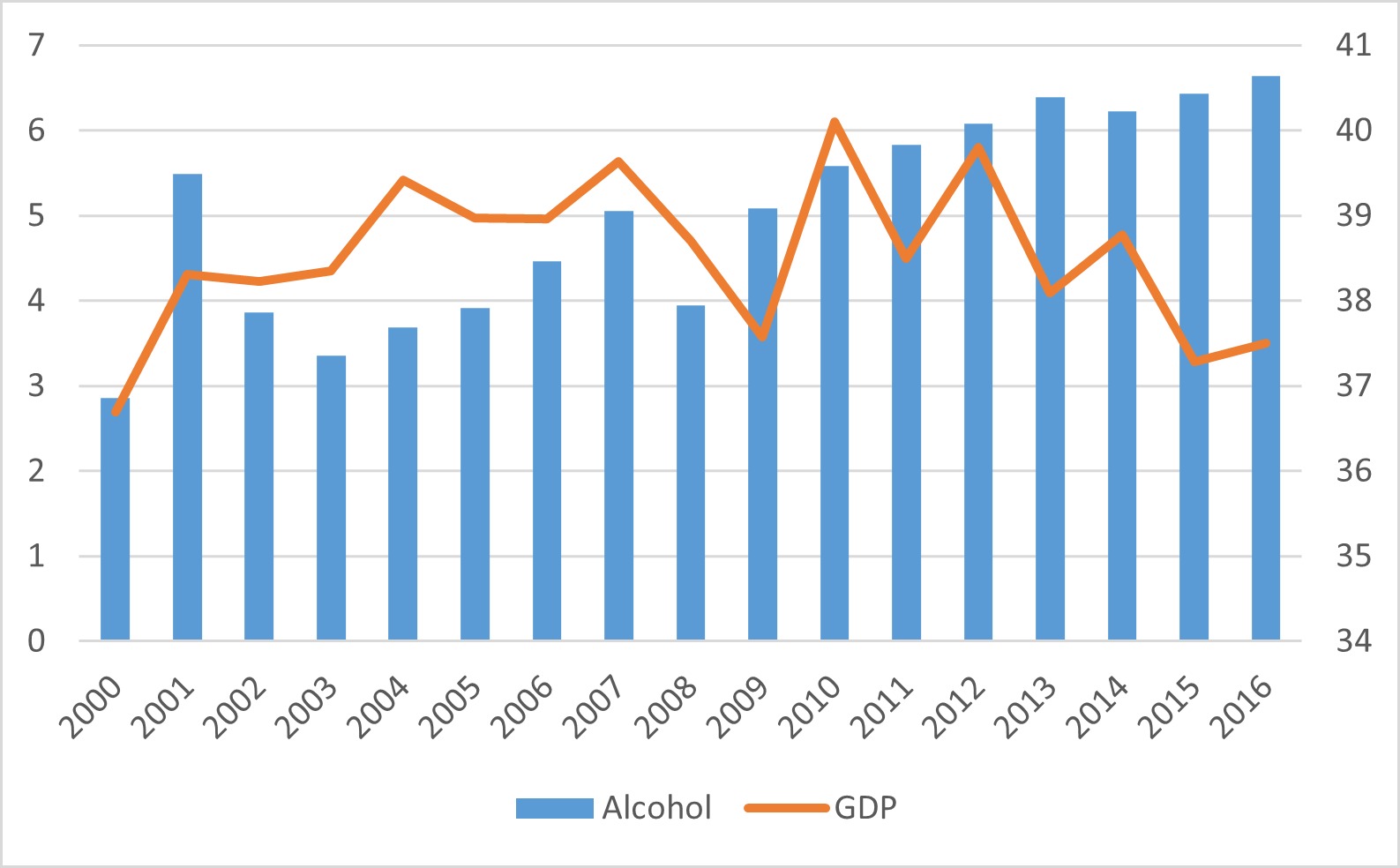
Furthermore,Odejide and Ibadan (2006) shows that the rate of alcohol consumption in Africa is increasing significantly. This is the reason why many studies have focused on the question of whether there is a threshold for alcohol consumption likely to influence consumer behavior on a social and even family level (Day, 1997; Ernhart et al., 1987; Hingson, Zha, & White, 2017; Pearson, Dawe, & Timney, 1999; Savolainen, Liesto, Männikkö, Penttilä, & Karhunen, 1993; Skinner, Glaser, & Annis, 1982; White, Kraus, & Swartzwelder, 2006; Wilson, O'Brien, & MacAirt, 1973; Wurst et al., 2003). In this regard,White et al. (2006) show through a logistic regression on students consuming alcohol in the USA that the higher this threshold, the greater the consequences. However, there is hardly any work that has determined the threshold for alcohol consumption concerning growth. This is why this study places at the heart of its problem whether there is a threshold effect of alcohol consumption compatible with the evolution of economic growth in sub-Saharan Africa. Indeed, this question is justified because we observe an ever-increasing demand for alcoholic products in sub-Saharan Africa, as shown in Figure 1 while economic growth does not seem to follow, especially since 2010. However, it is admitted that the beverage sector occupies a considerable place in public revenue, which, through production, is supposed to boost economic growth. Therefore, the objective of this paper is to determine the alcohol consumption threshold from which we would observe an opposite effect on economic growth. To achieve this objective, we use a non-linear threshold-effect model on a sample of 32 countries in sub-Saharan Africa over the period 2000-2016. We show through the ARDL estimator that there is no threshold effect on economic growth in the short run, but in the long run, we detect a threshold of $ 255.5, from which an increase in consumer demand for alcohol harms economic growth. This is evidence of an inverted U-shape curve between the demand for alcohol consumption and economic growth.
Literature review
In this section, we make an empirical review of the works on the threshold for alcohol consumption on the one hand and, on the other hand, on alcohol consumption in sub-Saharan Africa.
Concerning the threshold effect, the literature is quite extensive (Connor & Hall, 2018; Day, 1997; Ernhart et al., 1987; Hingson et al., 2017; Pearson et al., 1999; Savolainen et al., 1993; Skinner et al., 1982; White et al., 2006; Wilson et al., 1973; Wood et al., 2018; Wurst et al., 2003).Day (1997) determined the threshold at which alcohol consumption causes disease. He found that above 7 to 13 liters of alcohol consumed per week, women are at high risk of disease compared to men, for whom the threshold is 14 to 27 liters of alcohol. Moron et al (1987) found that consuming more than 3 liters of alcohol per day leads to neonatal abnormalities.Skinner et al. (1982) showed a threshold above which an individual can be considered an alcoholic and demonstrated that the probability of an individual considering himself an alcoholic increases with the degree of alcohol consumption. This is howWilson et al. (1973) measured the taste threshold for alcohol consumption in a sample of 173 subjects with an average age of 27 years. He found that this threshold varies between 15.1% and 22%. In addition, (O'Leary & Schumacher, 2003) studied the threshold for the degree of alcohol consumption likely to lead to domestic violence. White et al. (2006) showed that the higher the threshold for alcohol consumption by students, the greater the consequences. They found that on average, one in five men drinks more than 10 beers while one in 10 women drinks more than 8 beers.Savolainen et al. (1993) seek the threshold of ethanol use beyond which the effects are damaging on alcohol consumption and realized that the injection of ethanol in men over 25 years at a dose greater than 40 g increases this risk.Hingson et al. (2017) seek the threshold beyond which alcohol consumption negatively impacts the performance of occupations such as driving.
Regarding the work specific to Africa, the majority of these relate to the effects of alcohol consumption on health (Agyemang, Boatemaa, Frempong, & Aikins, 2015; Asiimwe et al., 2015; Ferreira-Borges et al., 2016; Granich, 2018; Kiene & Subramanian, 2013; Obot, 2006; Odejide et al., 2006; Roerecke et al., 2008). For example, (Agyemang et al., 2015) Kannan discovered that women who consume alcohol had a 1.37-fold increased risk of becoming overweight compared to those who do not (Hahn et al., 2012) showed that heavy alcohol consumption in Africa promotes transmission and at the same time, complicates the treatment of HIV / AIDS infection. Thus,Asiimwe et al. (2015) showed that people infected with HIV / AIDS tend to underestimate their spending and level of alcohol consumption. (Roerecke et al., 2008) showed that alcohol consumption was responsible for 2.2% of deaths in Africa in 2002. (Ferreira-Borges et al., 2016) estimated this rate at 6.4% in 2012 with a higher risk in people who have HIV / AIDS. (Ferreira-Borges et al., 2017) proposed reducing this death rate by acting on specific indicators such as the availability of alcoholic products and the fight against illicit production.
However, almost no study has looked at determining the threshold for alcohol consumption concerning growth. This lack justifies the interest of the present research.
Data and methodology
Data
We look at data from the WDI and WGI for a panel of 32 African countries from 2000 to 2016. Due to data availability limits, the periodicity and nations under inquiry were chosen. Table 1 below has a detailed overview of the data.
Table 1
Summary statistics
Table 1 shows that the maximum per capita amount annually spenton the alcohol consumption in our sample is 218.03 $ while the minimum amount is 0.39$. The first value corresponds to the amount spent in Burkina Faso for 2016 while the second is related to the amount spent in Niger for the year 2000. Concerning the Gross Domestic Product, the maximum value was recorded in Chad in 2004 (33.63), a few years later after the exploitation of their oil, while the lowest value of the GDP among the sample belonged to the Central African Republic in 2013 (-36.04). This level of growth was recorded during their recent period of political instability.
Table 2
Pairwise Correlation
The dependent variable is corruption, which is quantified in terms of GDP . Alcohol use is the most important independent variable . This study includes five control variables to limit the possibility of bias due to variable omissions. They are I open commerce, (ii) inflation, (iii) the internet, (iv) the active population, and (v) education. Table 1 shows the summary statistics for the variables, while Table 2 shows the Pairwise correlation analysis. The supplementary file contains a full discussion of variables as well as their definitions.
Methodology
This study employs the neoclassical enhanced growth model created by Mankiw, Romer, and Weil (1992) to examine the influence of alcohol consumption on economic growth. Taking into account the dependent variable (alcohol consumption), as well as the heterogeneity of the coefficients and other control variables, the model can be constructed as follows:
Where
The transformation of Equation
With
Where
Employing (Evans, 1997; Lee, Pesaran, & Smith, 1996; Pesaran & Smith, 1995; Pesaran, Shin, & Smith, 1999) Pooled 'Mean Group (PMG) technique, dynamic heterogeneous panels may be estimated
Equation (2) is rewritten as follows:
We conducted two stationary tests: the test of (Levine, Lin, & Chu, 2002) and (Im, Pesaran, & Shin, 2003; Kao, 1999).
Empirical results
The result of the stationary tests is recorded in Table 3. It is apparent from this table that the Gross Domestic Product and Inflation variables are stationary at level whereas the rest of the model variables are stationary in first difference.
Table 3
Results of stationary tests
Table 4 displays the results of theKao (1999) cointegration test. This table indicates that the model's variables are cointegrated if the probability of their cointegration is less than 5%.
The results of the stationary and cointegration tests allow us to use the PMG method to estimate the parameters of our growth model. The results of the growth model are recorded in Table 5.
Table 5
Regression of alcohol consumption on economic growth
Estimating growth equations using the PMG technique demonstrates that speed of adjustment is negatively significant for all models, supporting cointegration and suggesting that the tie between economic growth and explanatory variables is characterised by predictability.
This shows that the drinking of alcohol has no immediate impact on growth. However, in the long run, it has a beneficial and considerable impact on the economy (Column 6). Thus, an increase in alcohol consumption of one unit will lead to an increase in growth of 5.11 % in the long run. The tax revenue can explain this result on alcohol industries, which is one of the major sources of income for African countries. These incomes finally contribute to the formation of the GDP. The finding that alcohol consumption fosters economic growth is relatively not consistent with Thavorncharoensap, Teerawattananon, Yothasamut, Lertpitakpong, and Chaikledkaew (2009) who have found that alcohol has a significant economic impact on society. Results from the nonlinear specification show that the non-linear coefficient has a statistical influence on economic growth for the six equations. According to the empirical evidence, there is a threshold at which better-quality alcohol has a positive influence on economic growth, and above which it has a negative effect. An inverted U-shape is also apparent from the evidence (Laffer curve of alcohol). The control variables have the expected signs. Trade, active population and education have the expected positive sign while inflation and the internet are expected negative. Moreover, we find the threshold value beyond which an increase of one unit of alcohol would drop the economic growth by solving the equation
This value is obtained as:
Using the latter formula, we found that the threshold value of alcohol consumption per capita is 255.5 $ (column 6). This result can be explained by the fact that the overconsumption of alcohol will surely increase the tax revenue perceived by the States. However, this situation will hamper the productivity of the labour factor, which is very important for the production system. At this level, the amount of taxes lost on the overall production system will be more than that of tax perceived on alcohol consumption by the States. This result is compatible with the empirical literature, which demonstrates the existence of a threshold beyond which alcohol consumption leads to disease (Asiimwe et al., 2015; Granich, 2018); negatively influences professions such as driving (Hingson et al., 2017) and leads to death (Roerecke et al, 2008; Ferreira et al, 2017). All these negative aspects of overconsumption of alcohol hamper economic growth. This result is also consistent with Thavorncharoensap et al. (2009), who have found that alcohol has a significant economic impact on society.
In order to test the robustness of the above results, we introduced other control variables (employment, foreign direct investment and government effectiveness) in the model, and we also used an alternative estimation technique. The estimation of this model is the Generalized Moments Method system of Blundell and Bond (1998). Besides the endogeneity problem, this method is also robust to autocorrelation and heteroskedasticity. It also corrects the problem of variables omitted from the model. The validity of the result produced is based on two main tests: the second-order autocorrelation test and the conformity test of Sargan's overidentification test (1958). The results of the GMM estimation are recorded in Table 6.
Table 6
GMM estimation with more control variables
The analysis of the effect of alcohol consumption on economic growth by the GMM system shows that the wald test is significant at 1% for all models, which means that the models are well specified. In addition, we observe an absence of second-order autocorrelation at the 5% threshold and the validity of the instrument identification test in four columns. The results also show that economic growth lagged by one period has a positive and significant effect on economic growth at the 1% threshold. This result corroborates the convergence theory of the growth model of Barro (1990), which states that the economic growth levels of different economies tend to be a loser over time. Alcohol intake has a positive effect on economic growth when consumed in moderation, but when consumed in excess, it has a negative effect on growth. The evidence points to a U-shape that is inverted (Laffer curve of alcohol). Moreover, foreign direct investment and government effectiveness variables foster economic growth, whereas employment variables have no significant effect on economic growth (column 4).
Conclusion
This study added to the body of knowledge by examining the nonlinear link between alcohol consumption and economic growth in 32 African countries between 2000 and 2016. The alcohol consumption expenses per capita are used to capture the alcohol variable. The empirical evidence is based on PMG and GMM. The results show that: (i) alcohol consumption fosters economic growth in sub-Saharan African countries, and (ii) there exists a non-linear relation between alcohol consumption and economic growth. The empirical evidence shows that there is a threshold at which increasing alcohol use has a positive influence on economic growth and a negative effect over this threshold. An inverted U-shape is also apparent from the evidence (Laffer Curve of alcohol). As a result, governments in Sub-Saharan Africa are working to limit the amount of alcohol that their citizens consume in order to keep them safe from alcohol-related ailments while also ensuring the region's long-term economic viability.